Hypothesis Testing

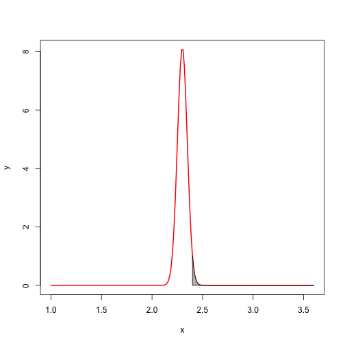
Let \(X\) be a normally distributed data with mean \(\mu\) and standard deviations \(\sigma\). Symbolically, it is writen as \(X \sim N(\mu, \sigma^2 )\).

Any normally distributed data can be tranferred into a special type of normal distribution called "standard normal distribution". The transferred random variable is denoted by \(Z\). The tranformation formula:

\(Z= \frac{(X- \mu )}{\sigma }\)

where \(Z\sim N(0,1)\).

A simplified version of z-transformation can be written as

\(Z= \frac{(data- mean)}{standard deviation}\)

where mean and standard deviations are population parameters.

1. A car manufacturer advertises that its new subcompact models get 47 miles per gallon(mpg). Let \(\mu\) be the mean of the mileage distribution for these cars. You assume that the manufacturer will not underrate the car, but suspect the mileage might be overrated.

• Manufacturer's claim is called null (status-quo) hypothesis. It is denoted by \(H_{o}\)
• Your suspicion (the car might be overrated ) is called an alternate hypotheis. It is denoted by \(H_{A}\)

1. Hair and cancer: Suppose a certain hair dye is to be tested to determine whether it is carcinogenic(cancer causing). The dye will be painted on the skins of 20 mice (group 1), and an inert substance will be painted on the skins of 20 mice (group 2) that will serve as controls. The observation \(X\) will be the number of tumors apprearing on each mouse.
   • What is the null Hypotheis ? \(H_{o}: .....\)
   • What is an alternate Hypothesis ? \(H_{A}: .....\)

1. The resoning used in statistical test of hypotheis is similar to the process in a court trial. In trying a person for theft, the court must deide between innocence and guilt.

2. As the trial begins, the accused person is assumed to be innocent.

3. The procecuttion collects and presents all available evidence in an attempt to contradict the innocent hypothesis and hence obtain a conviction.

4. If there is enough evidence against innocence, the court will reject the innocence hypothesis and declare the defendant guilty.

5. If the procecution does not present enough evidence to prove the defendant guilty, the court will find him not guilty.

6. This does not prove that the defendant is innocent, but merely that there was not enough evidence to conclude that the defandat was guilty.

A statistical test of hypotheis is a procedure for assessing the strength of evidence present in the data in support of alternate hypothesis \(H_{A}\).

\[Z_{test}= \frac{(data- mean)}{Standard \quad error}\]

1.When data=\(\bar{x}\)

\(mean (\mu_{\bar{x}}) = \mu\) , sd (\(\sigma_{\bar{x}}\)) =standard error = \(\frac{\sigma }{\sqrt{n}}\)

\[Z_{test}= \frac{(\bar{x}- \mu )}{\frac{\sigma }{\sqrt{n}}}\]

2.When data = \(x\), where x is binomialy distributed r.v with probability of success \(p\).

mean \((\mu_{x})= np\); sd \((\sigma_{x})=\sqrt{npq}\)

\[Z_{test}= \frac{( x- np )}{\sqrt{npq}}\]

given

x: binomially distributed data(count)

n: number of independent binomial trials

p: probability of success in each trials

q = (1-p)

p+q=1

Sample propotion= \(\hat{p}= \frac{x}{n}\)
where, \(x\) is the number of success and \(n\) reprsents.

Population Proportion= \(p\)

total number of trial = \(n\)

\[Z_{test}= \frac{(\hat{p}- p )}{\sqrt{\frac{ pq}{n}}}\]

Conditions to be satisfied for the normal approximation to binomial:
\(n\hat{p}>5\) and \(n \hat{q}>5\)

1. In a courtroom, a defendant could be judged not guilty whe he/she's is really guilty
   

2. Similarly, a defendant could be judged guilty whe he/she's is not really guilty
   

There are two types of errors that can be made. The null hypothesis may be either true or false, regardless of the decision the experimenter makes.

• Type I Error is exactly same as level of significance $\alpha$ : P(Type I Error)= $\alpha$
• P(Type II Error)= P(Fail to reject $H_{o}$ when it is False). It is denoted by $\beta$

Compliment of Type II Error= P(Rejecting \(H_{o}\) when \(H_{o}\) is False)

Compliment of Type II Error= 1- P(Fail to reject \(H_{o}\) when it is False)

Compliment of Type II Error= 1- \(\beta\)

The quantity \(1-\beta\) is called the POWER of the test.

A random sample of \(n=35\) observatios from a quantitative population produced a mean \(\bar{x}= 2.4\) and a standard deviation \(s= 0.29\). Suppose your research objective is to show that the population mean \(\mu\) exceeds 2.3.

\(H_{o}: \mu>2.3\)

se= \(\frac{sigma}{\sqrt(n)}\)

#se= sd/sqrt{n}
 se= 0.29/sqrt(35)
 se

[1] 0.04901895

I assume you can find p-value and draw conclusion using p-value. Our goal here is to learn about power of the test.

Calculate the value(s) of \(\bar{x}\) corresponding to the border(s) of the rejection region. There will be one border value for a one-tailed test and two for a two-tailed test.

Boarder value for right tailed test (our example!) with 5% level of sigificance is the value of \(\bar{x}\) for given \(\alpha\), sample size and \(\sigma.\)

\(\bar{x}= \mu+z_{\alpha}\frac{\sigma}{\sqrt{n}}\)

xbar= 2.3+qnorm(0.95)*0.29/sqrt(35)
 xbar

## [1] 2.380629

\(\beta =P(accept H_{o}\) when \(\mu=2.4)\)

\(\beta =P(accept \quad H_{o} when \quad \mu=2.4) = p(\bar{x}< 2.380629)\)

We assume that the null hypothesis is false. This lead us to assume different value of \(\mu.\) Practically, \(\mu\) itself is random. We will find of the test for differnt values of \(\mu.\)

When \(\mu=1.9\)

 mu=1.9; n<- 35
 beta<-pnorm(2.380629, mean= mu, sd=0.29/sqrt(n)) # xbar=2.38
 beta

[1] 1

p=1-beta;p

[1] 0

 mu1=2.0
 mu1

[1] 2

 n<- 35
 beta1<-pnorm(2.380629, mean= mu1, sd=0.29/sqrt(n))
 beta1

[1] 1

p1=1-beta1
p1

[1] 4.107825e-15

 mu2=2.1
 mu2

[1] 2.1

 n<- 35
 beta2<-pnorm(2.380629, mean= mu2, sd=0.29/sqrt(n))
 beta2

[1] 1

p2=1-beta2
p2

[1] 5.174466e-09

 mu3=2.2
 mu3

[1] 2.2

 n<- 35
 beta3<-pnorm(2.380629, mean= mu3, sd=0.29/sqrt(n))
 beta3

[1] 0.9998856

p3=1-beta3
p3

[1] 0.0001144046

 mu4=2.3
 mu4

[1] 2.3

 n<- 35
 beta4<-pnorm(2.380629, mean= mu4, sd=0.29/sqrt(n))
 beta4

[1] 0.95

p4=1-beta4
p4

[1] 0.04999998

 mu5=2.4
 mu5

[1] 2.4

 n<- 35
 beta5<-pnorm(2.380629, mean= mu5, sd=0.29/sqrt(n))
 beta5

[1] 0.3463573

p5=1-beta5
p5

[1] 0.6536427

 mu6=2.5
 mu6

[1] 2.5

 n<- 35
 beta6<-pnorm(2.380629, mean= mu6, sd=0.29/sqrt(n))
 beta6

[1] 0.007441755

p6=1-beta6
p6

[1] 0.9925582

 mu7=2.6
 mu7

[1] 2.6

 n<- 35
 beta7<-pnorm(2.380629, mean= mu7, sd=0.29/sqrt(n))
 beta7

[1] 3.816477e-06

p7=1-beta7
p7

[1] 0.9999962

 mu8=2.7
 mu8

[1] 2.7

 n<- 35
 beta8<-pnorm(2.380629, mean= mu8, sd=0.29/sqrt(n))
 beta8

[1] 3.628283e-11

p8=1-beta8
p8

[1] 1

Let's plot power verses different values of \(\mu\).

mean<- c(mu, mu1, mu2, mu3, mu4, mu5, mu6,mu7, mu8)
power<- c(p, p1, p2, p3, p4, p5, p6, p7, p8)

plot(mean, power, col="blue")

Change in power of the test is more visible if we plot last five pairs data.

mean<- c( mu4, mu5, mu6,mu7, mu8)
power<- c( p4, p5, p6, p7, p8)

plot(mean, power, col="blue", type="o" , pch=19)